By Andrea Leccese
July 3rd, 2021
While investors are looking after the best investment managers, some also actively manage their investments by withdrawing money from the fund when markets decline and reenter when markets rally. In this report, we simulated different scenarios where investors actively manage their investment and calculated the investment performance accordingly to analyze whether it would bring a better return to investors.
Investment in an Active Investment Strategy without Withdrawal
To analyze whether investors could benefit from actively managing their investment into one portfolio, we choose one of our portfolios as an example in the analysis. Figure 1 shows the performance and the monthly return of a portfolio that actively managed by Bluesky Capital.
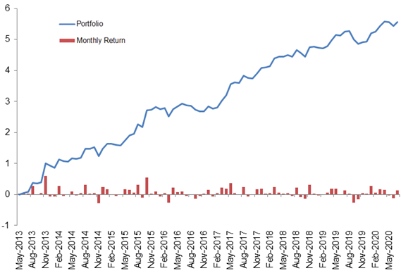
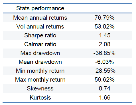
Table 1 shows the performance statistics of the portfolio that we choose as an example in our following analysis. The portfolio has an average annual return at 76.79% with a 1.45 Sharpe Ratio.
Time Series Analysis Active Investment Performance
As we were trying to simulate investment decisions made by investors who actively manage their investment, we conducted a time series analysis of the portfolio return to generate position signals. If the time series could provide some useful insights to guide investor in making decisions, we could then use those signals to do the simulations.
As time series models are based on mathematical assumptions, it’s necessary to check whether the data meet those assumptions before fitting any models and making predictions. Autocorrelation Function (ACF) and Partial Autocorrelation Function (PACF) are usually used in detecting patterns of the data in time series analysis. Figure 2 shows the ACF and PACF from lag 0 to 20 of the portfolio return with 95% confidence intervals. We could see that ACF and PACF of the portfolio return are not significant, indicating that the return itself is a white noise. In other words, the original data provide us little information for forecasting.

Portfolio Performance with Timing
As mentioned in section 2 that we couldn’t use the original return data directly to generate an investment position signal, we use a simplified signal to simulate investors’ investment decisions. We assume that investors would withdraw their money from a fund or a portfolio when the sum of returns during a specific previous window is negative and would reinvest when the sum of returns turns to positive. Therefore, the position would be 1 if the sum is positive, meaning invest into the portfolio. Otherwise the position would be 0, indicating a withdrawal from the portfolio. For example, Portfolio Lag 1 means that the investor would withdraw from or reinvest into a portfolio based on the portfolio return of the previous month.
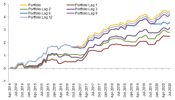
Figure 3 shows the simple cumulative return of the portfolios with different lags. Investors who invest into the portfolio without any withdrawals during the study window would get the highest return.
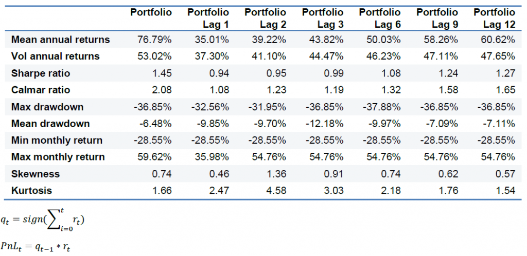
Table 2 shows the performance statistics of different portfolios. The average annual return increases as the looking back period (the lag) becomes longer. While the volatility of the Portfolio Lag 1 is the smallest among the portfolios, the Sharpe Ratio of the Portfolio Lag 1 is the lowest. The reason that the volatility of the Portfolio Lag 1 is smaller than others is that the investors actively withdraw money from the portfolio when performance declines. However, such investors sacrifice their investment return in the meantime. Investors who didn’t withdraw their money during the whole period would enjoy the highest risk-adjusted return.
Conclusion
The previous results highlight the following key insights:
- The portfolio historical return itself could not provide insightful information in generating investment position signals: The autocorrelation and partial autocorrelation analyses of portfolio return show that the return itself is a white noise. Without data engineering or transformation, the portfolio historical return could provide investors little information in forecasting. If it could, the investment manager would have probably already exploited it to generate better returns for his clients.
- Investors would get higher risk-adjusted investment returns when they don’t try to time their investments in an actively managed portfolio: investors who keep their money in the portfolio during our study’s timeframe receive the highest risk adjusted return with a Sharpe Ratio 1.45. Although investors who actively manage their investment may achieve a lower volatility by withdrawing money from the portfolio, they would miss some return as well and would have the lowest Sharpe Ratio at 1.08. It is therefore important to stick with your portfolio manager for the long-run.
Subscribe to our newsletter to receive our latest insights in quantitative investment management. For more info about our investment products, send us an email at info@blueskycapitalmanagement.com or fill out our info request form.