By Alyssa Wei
June 28th, 2021
This research article analyzes the influences of determinant macroeconomic factors – GDP, GDP Surprise, Inflation, and Inflation Surprise – on asset returns and asset correlations. In particular, we analyze how the previous factors impact the performance of different investment portfolios during various phases of the economic cycle. We found that portfolios that show the highest risk-adjusted and most robust returns with respect to different economic conditions are the ones that are invested across multiple asset classes that have offsetting responses with respect to the macro factors analyzed.
The article is structured as follows. The first section analyzes the influences of GDP growth and inflation on asset returns. The second section further analyzes such impacts using regression models. The third section compares the performance of three different portfolios, including the benchmark 60/40, the minimum variance, and risk parity portfolios. The fourth section analyzes if changes in macroeconomic factors affect changing correlations among asset classes over time. The last section concludes with key takeaways.
Influences of GDP Growth and Inflation on Asset Returns
Portfolio diversification is of great importance for investors in achieving investment goals while managing risks. However, a diversified portfolio across asset classes doesn’t guarantee diversified risk exposures. Macroeconomic factors, such as GDP growth and inflation, have impacts on financial markets. Therefore, how to diversify and minimize risk exposures of a portfolio to macroeconomic factors would be a worthwhile research to do for investors and portfolio managers. In the following sections we will discuss the relationship between financial assets and macroeconomic factors. Our analysis will mainly focus on GDP and inflation, as these macroeconomic factors are usually considered the most important with respect to the performance of different asset classes. Table 1 shows indices and data used in our analysis. Figure 1 and Figure 2 shows the assets prices and scaled assets prices from January 1970 to January 2019.
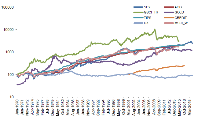
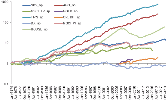
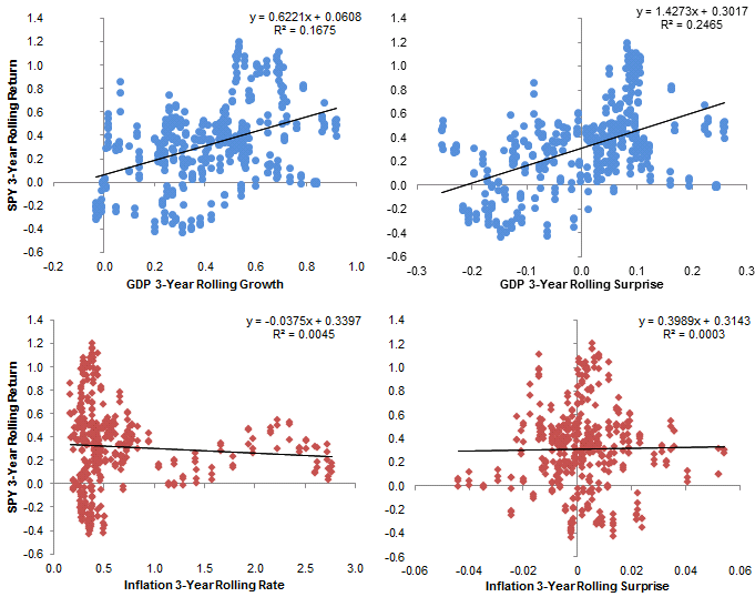
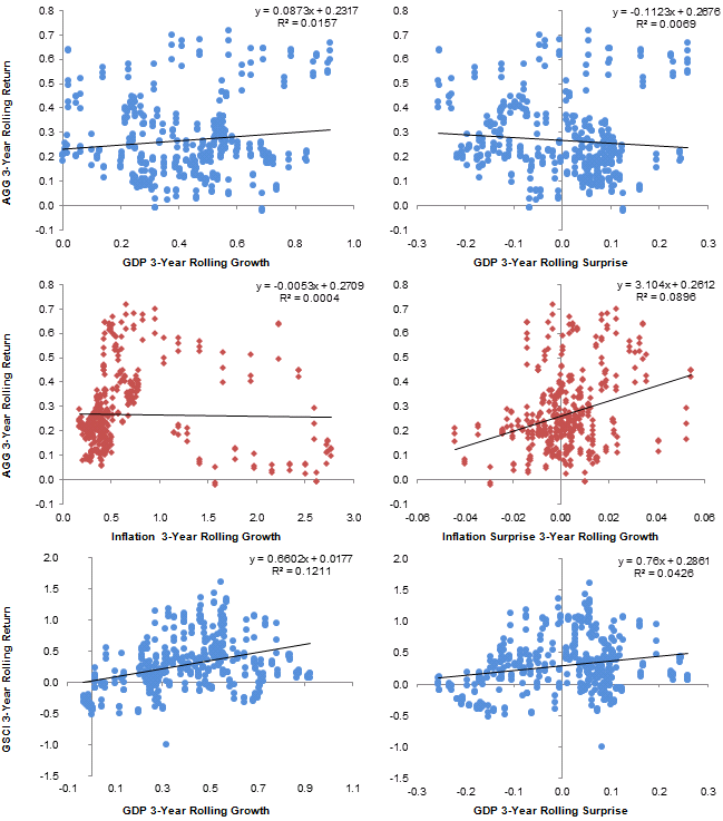
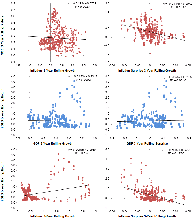
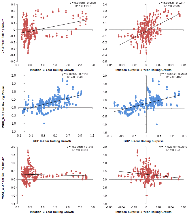
As index values are different in magnitudes (Figure 1), the asset prices scaled by rolling 5-year volatility in Figure 2 provide a more accurate information about the performance of different asset classes. TIPS index increased strikingly compared to other assets. After checking the trend of price, we plot asset returns against factors that we are interested in — GDP, GDP surprise, Inflation and Inflation Surprise (Appx A). The scatter plots verify our initial thoughts about the influence of GDP and inflation on asset returns. For example, after rolling data by 3 years, 16.75% and 24.65% of the variation in the SPY rolling returns could be explained by the GDP growth rate and the GDP surprise respectively. Compared to GDP, inflation and inflation surprise have limited explanatory ability on the variation of SPY returns. Such result is in line with our expectations that economic growth and uncertainty of future economy are built into the prices of equities.
Regression Analysis of Impacts of Factors on Asset Returns
To further analyze the relationship between macroeconomic factors (GDP growth and inflation) and other asset returns, we conduct a linear regression analysis by setting the asset monthly returns as the dependent variables. For every asset, we build linear regression models using GDP, GDP surprise, Inflation and Inflation surprise as the independent variables respectively. Table 2 shows the results of the regression.
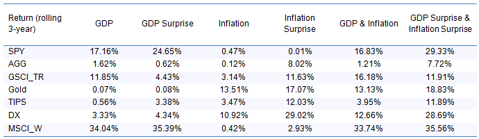
As mentioned in the previous section, GDP and GDP Surprise have higher explanatory power on variation of SPY return (3-year rolling) than inflation or inflation surprise does. A similar result also holds for the regression analysis on MSCI World Index (MSCI_W). GDP and GDP Surprise have much higher R^2 than inflation does. Inflation and inflation surprise, on the other side, have higher impact on Gold price, with R^2 at 13.51% and 17.07% respectively. In general, regression models that include both GDP and inflation have higher R^2 than simple linear regression models with only one factor as we would expect. In summary, GDP and inflation do have influence on asset returns, while the degree of impact is different across assets. Equities are more sensitive to GDP growth. Assets such as Fixed Income (AGG), Currency (DX), and Gold are more sensitive to the inflation rate, in line with macroeconomic intuition. Specifically, commodities (GSCI_TR) have sensitivity to both GDP and inflation surprise. Inflation protected bonds (TIPS) have lower sensitivity to GDP, GDP surprise and inflation, but higher sensitivity to inflation surprise.
In addition, we interest in the market reactions to the GDP Surprise and Inflation Surprise. To analyze effects of surprises, we further conduct regression analysis based on a 5-year window of data. By using sliding windows, we could observe a list of regression coefficients, including alpha (the intercept: the excepted return of an asset without any GDP or Inflation Surprise), betas for GDP and Inflation (the change in expected asset return along with per unit change in GDP or Inflation Surprise). For illustration purpose, we plot a 20-month moving average value of coefficients to make the line smooth (Figure 4)
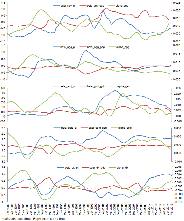
From Figure 4, we could spot that GDP Surprise and Inflation Surprise tend to have opposite impact on asset returns, as the beta of GDP Surprise (red line) and beta of Inflation Surprise (blue line) move in opposite directions. The changes of coefficients provide some information about the economy environment. Taking AGG as an example, the betas for AGG are close to zero starting from September 2008, which may because of the $4 trillion quantitative easing program and the low interest rate during that period. The return of bond investments becomes low and more independent from macroeconomic factors. This could be one of the reasons for near zero betas for AGG. Another example of coefficients reflecting the economy would be DX (Dollar Index). While alpha for other assets are positive, we notice several negative alpha period for DX, which accords with the FX market, as neither long nor short only position could bring return.
Portfolio Performance with Respect to Different Macroeconomic Cycles
In this section, we compared the performance of three different portfolios to see which one performs better with respect to different macroeconomic cycles when we only consider inflation and GDP as the dominant factors. The portfolios are static weighted 60/40 portfolio, minimum variance portfolio and risk parity portfolio. The 60/40 portfolio invests 60% in the equity market, as represented by the S&P 500 (SPY) and 40% in the bond market, as represented by the Barclays Aggregate Bond Index (AGG). This portfolio is typically held by institutional investors, which is usually considered as a diversified portfolio and used as a benchmark. The minimum variance portfolio and the risk parity portfolio invest in equities (SPY), bonds (AGG), commodities, and inflation protected bonds. The commodity market is represented by S&P GSCI Commodity Total Return (GSCI_TR) and the inflation protected bond is represented by Bloomberg Barclays US Treasury Inflation Notes TR Index (TIPS). The min variance aims at achieving lower portfolio volatility, while the risk parity focuses on allocation of risk. The risk portfolio is built in a way such that each asset has an approximately 25% risk contribution to the portfolio. Figure 5 shows the cumulative returns of those three portfolios from March 1976 to April 2015.
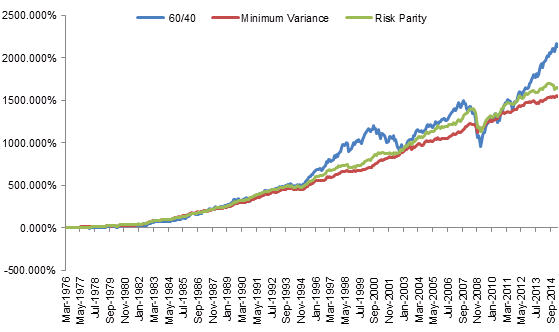
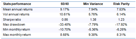
By April 2015, The 60/40 portfolio has the highest cumulative returns among the three portfolios, as it has the highest investments weights in the equity, which is 60%. On the other hand, the 60/40 portfolio also shows a high volatility compared to the other two portfolios, as it is less diversified. Therefore, the 60/40 portfolio achieves a higher cumulative return at the expense of bearing more risk. From Table 3, we could notice that although 60/40 portfolio has the highest average annual returns at 9.17%, however, it has the lowest Sharpe ratio 0.86, indicating a low return per unit of risk taken. The good performance of min-variance portfolio and risk parity portfolio in terms of Sharpe ration is because of diversification of the assets allocation.
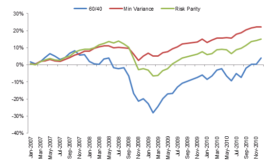
The advantages of a well-diversified portfolio would be easier to detect during financial crisis period. Figure 6 shows the cumulative returns of the three portfolios from January 2007 to December 2010. The maximum monthly loss of 60/40 portfolio would have happened in February 2009 with 28.04% loss in that month; meanwhile the return of min-variance portfolio and risk parity portfolio would be 5.15% and -6.57% respectively. The lowest monthly return of min-variance portfolio was 0.347% in February 2007 and the lowest monthly return of risk parity portfolio was -6.57% in February 2009. The min-variance portfolio, which targets at minimizing the portfolio volatility, has a better performance during the financial crisis among the three portfolios.
In terms of drawdown, diversified portfolio also has a better performance. Figure 7 shows the drawdown of 3 investment portfolios from March 1976 to April 2015. The 60/40 portfolio has a high drawdown in general compared to the other two portfolios. As the 60/40 portfolio has a high risk exposure to the equity market, the portfolio has a high volatility.
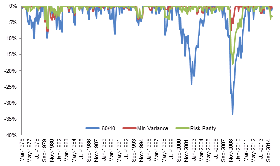
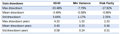
Table 4 shows the drawdown statistics for the 3 investment portfolios. The min-variance portfolio has the lowest and fastest to recover drawdowns, followed by the risk parity portfolio. The min-variance portfolio also has the lowest max drawdown 7.79%, which is almost half of the max drawdown of risk parity portfolio and one quarter of 60/40 portfolio. In reference to our analysis in section 1 and section 2, where we found that macroeconomic factors have different levels of impact on financial assets, a multi-asset portfolio would have mitigated the risk exposures to different economic cycles.
In conclusion, based on the previous results, a diversified portfolio, such as the min-variance portfolio and the risk parity portfolio, outperforms the traditional 60/40 portfolio, providing a much less risk per unit of return. Investing in the min-variance portfolio reduces drawdown width and length and improves the Sharpe ratio, at the expense of less mean annual returns.
Influences of Macroeconomic Factors on Dynamic Correlations among Asset Classes
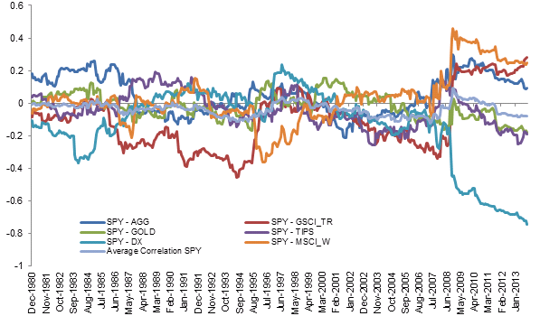
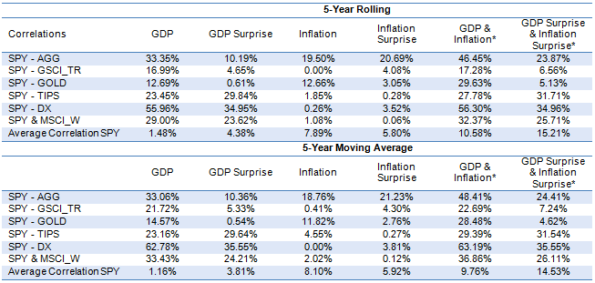
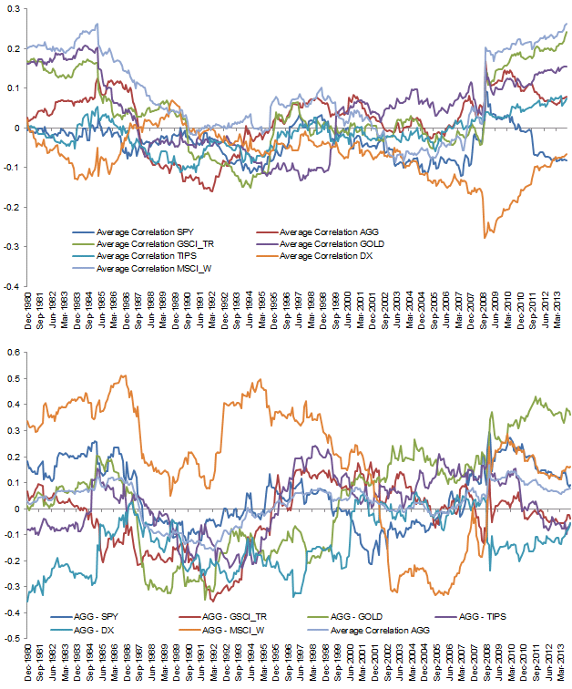
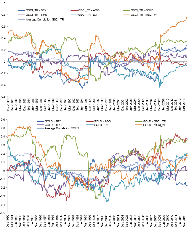
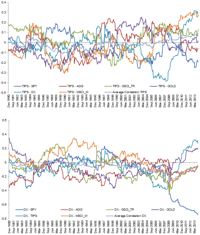
While building a multi-asset portfolio, one should also keep the correlation across asset classes in mind. A portfolio with extremely positively correlated assets would have a high volatility of portfolio return, as asset prices would move in the same direction. Figure 8 Rolling 5-Year Correlations of SPY and other assets show the rolling 5-year correlations of SPY and other assets (Appx B) includes charts of correlations for other assets). The Average Correlation SPY is the average value of correlations between SPY and the other assets. From March 1976 to around June 2008, the across asset correlation between SPY and other assets are in the range of -0.2 to 0.2. However, assets became more correlated during and after financial crisis in 2008. For example, the correlation between SPY and DX increased to -0.45 by the end of December 2008.
As Figure 8 shows, the correlations among assets are not static. We then further analyzed whether factors, such as GDP growth and inflation, could explain the changes of the correlation between two assets. Table 5 shows the results of the regression analysis. Compared to the regression in section 2 (Table 2), GDP, inflation and their related factors have much higher explanatory abilities on correlations across asset classes than on the asset returns. When using a single factor to explain the changes in correlations, GDP and GDP surprise show higher R^2 than inflation and inflation surprise do under most cases. Moreover, the variation of correlations could be explained better by using two factors than a single factor, indicating that GDP and inflation together have impact on the variation of correlations.
Conclusion
The previous results highlight the following key takeaways:
- Macroeconomic factors — GDP, GDP Surprise, Inflation and Inflation Surprise — have high impact on asset returns: the variation of asset returns could be explained by macroeconomic factors mentioned above. The explanatory ability is different across assets. While equities are sensitive to economic growth, bonds have a high exposure to inflation and inflation surprise compared to economic growth.
- Diversified portfolios, such as min-variance portfolio and risk parity portfolio, have better risk-adjusted performance than traditional 60/40 portfolio across different macroeconomic cycles: traditional 60/40 portfolio is not diversified enough in terms of risk exposures, which is highly vulnerable to equity related risks. Through increasing the asset diversification of a portfolio, a better portfolio performance could be achieved. The Sharpe ratios of min-variance portfolio and risk parity portfolio are higher than the ratio of 60/40 portfolio by approximately 0.6 and 0.4 respectively. They also more resilient than 60/40, with shallower drawdown during and quicker recovery from financial crisis. During our backtested period, the max drawdown of min-variance portfolio is 7.79% and of risk parity portfolio is 17.92%, compared to 33.48% of 60/40 portfolio.
- Correlations between asset classes are not static and macroeconomic factors have explanatory ability towards the variation of correlations over time: we notice an apparent increase in correlations among asset classes during financial crisis, suggesting the importance of resilience of portfolios during turbulent market environments. Our analysis shows that asset classes have different exposures to GDP growth and inflation. Moreover, the sensitivities to GDP or GDP surprise and to Inflation or Inflation surprise are different as well. By analyzing impacts of factors on asset correlations, investors could build portfolios that are more resilient to different economic cycles, which may provide higher risk-adjusted returns over the long term.
Appendix A: 3-Year Rolling Asset Returns vs. Macroeconomic Factors
Appendix B: Rolling 5-Year Correlations of Assets
Subscribe to our newsletter to receive our latest insights in quantitative investment management. For more info about our investment products, send us an email at info@blueskycapitalmanagement.com or fill out our info request form.